Crafting Publication Quality Data Visualizations with ggplot2

Eric R. Scott

Learning Objectives

• Customize color palettes with accessibility in mind
• Customize legends
• Customizing axes (titles, labels, breaks)
• Customize appearance of plots with themes
• Arrange multi-panel figures
• Save high resolution or vector formats

Required Packages

library(tidyverse) #includes ggplot2
library(palmerpenguins) #for data
library(patchwork) #multi-panel figures
library(colorspace)

Take a moment to check if these load and install them if you need to.

Journal Requirements

Journals often require certain modifications to your plots to make them publication-ready

• High resolution
• Specific file types (TIFF, EPS, PDF are common)
• Figure size limits
• Font size suggestions

Get audience suggestions before advancing bullets

Not required, but good practice

Other modifications to the appearance of your plot are a good idea, but less often required by journals or reviewers

• Colorblind accessible colors
• Grey scale friendly colors
• Perceptually-even colors
• Screen-reader compatible
• High data-ink ratio (simplify plot, within reason)
• Arrangement of related plots into multi-panel figures

Get audience suggestions before advancing bullets

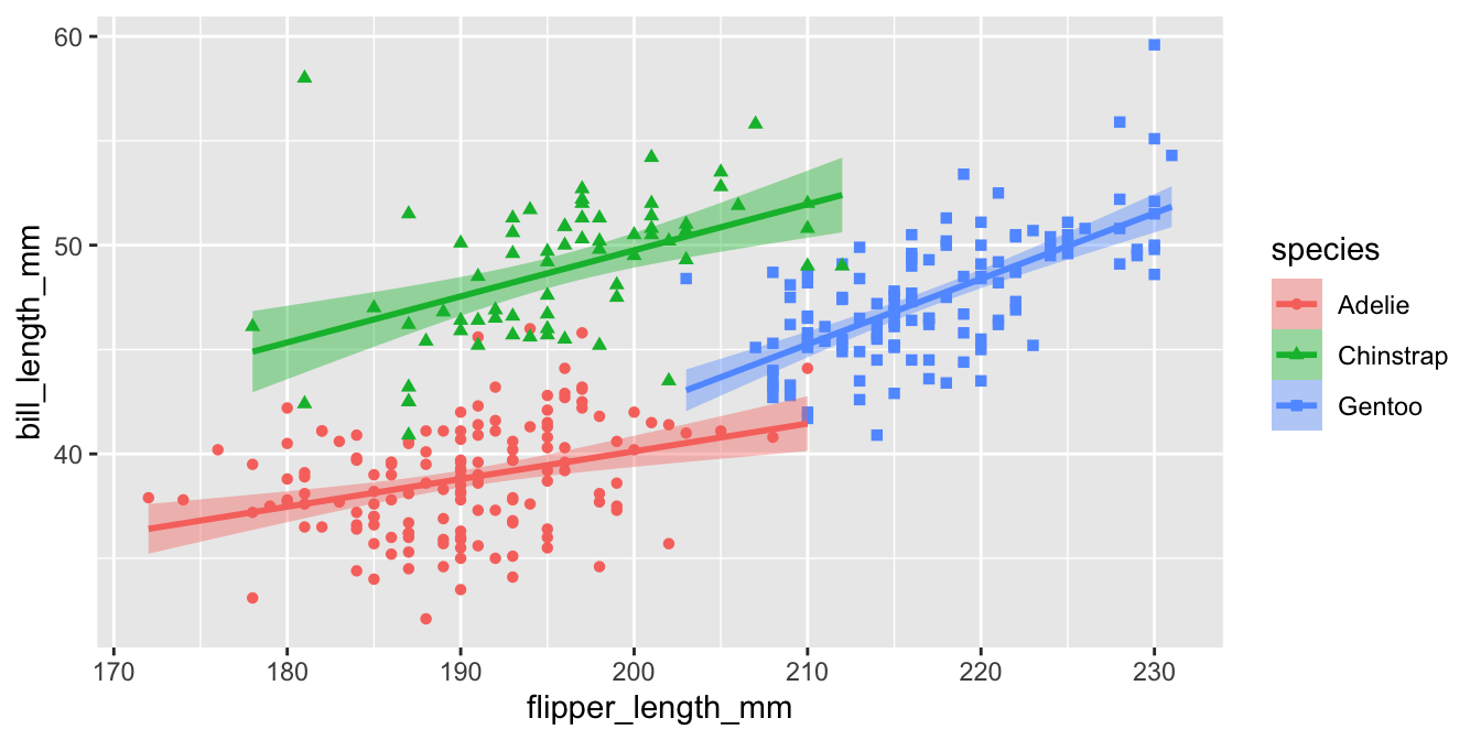
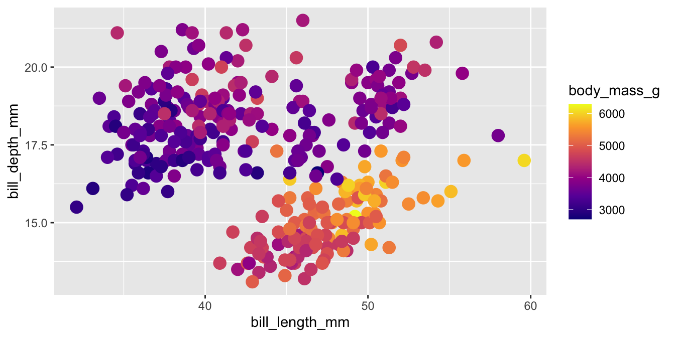
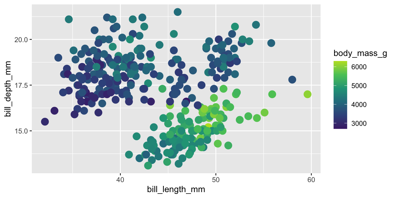
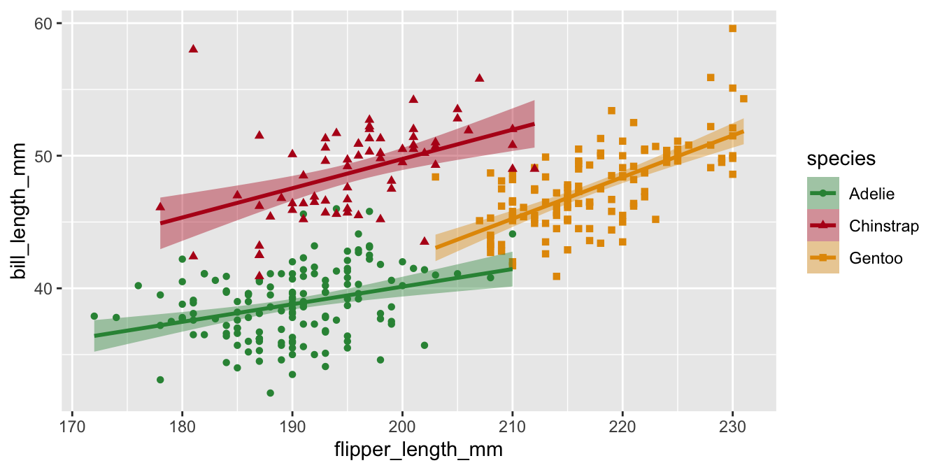
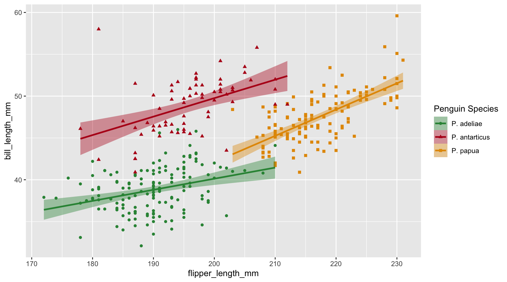
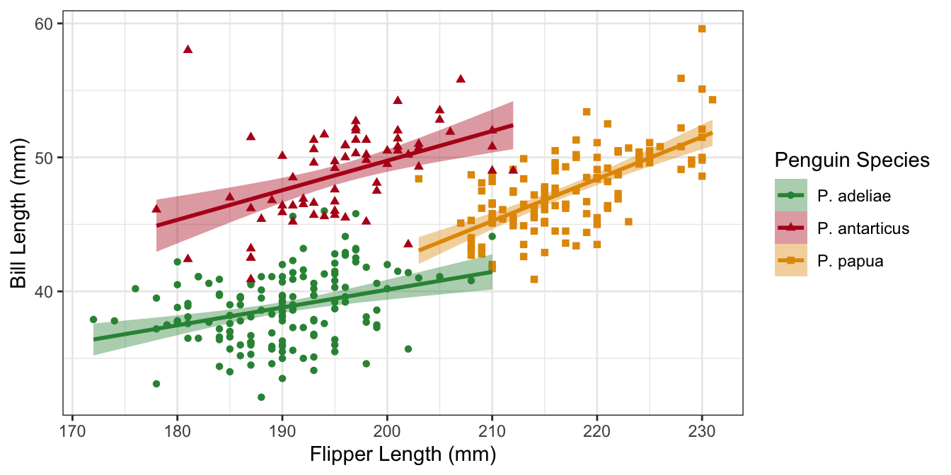
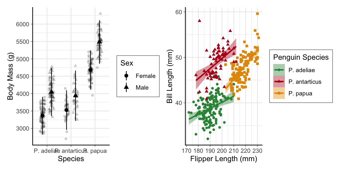
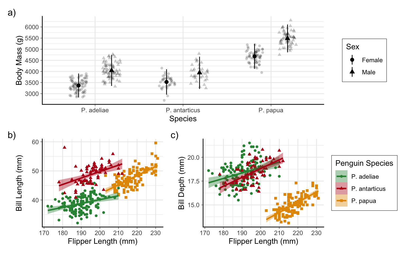
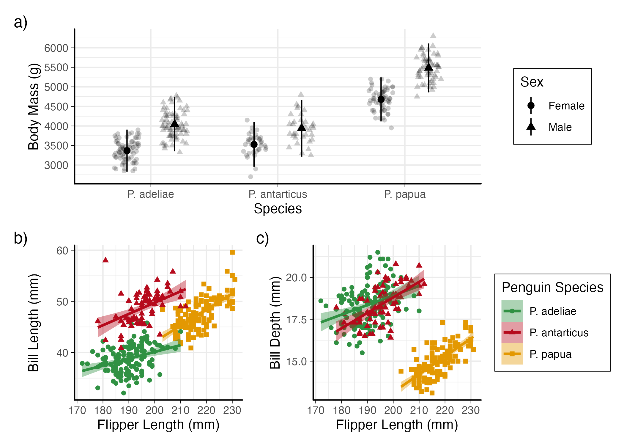
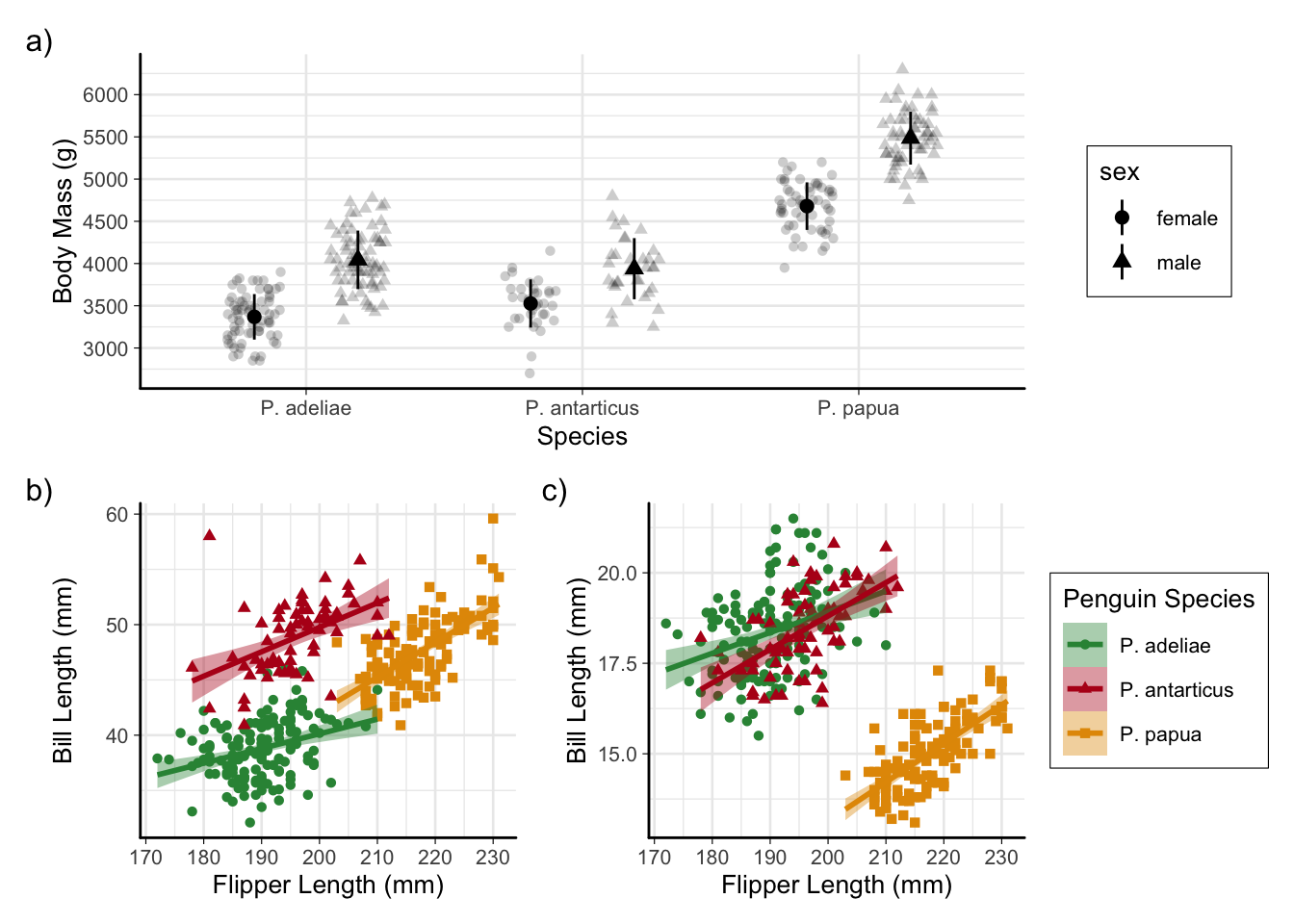
Example plot 1

p1 <-
  ggplot(penguins |> filter(!is.na(sex)),
         aes(x = species, y = body_mass_g, shape = sex)) +
  geom_point(alpha = 0.2,
    position = position_jitterdodge(dodge.width = 0.75)) +
  stat_summary(fun.data = mean_sdl,
    position = position_dodge(width = 0.75))
p1

Walk through construction of basic plots briefly. Encourage students to copy and paste code.

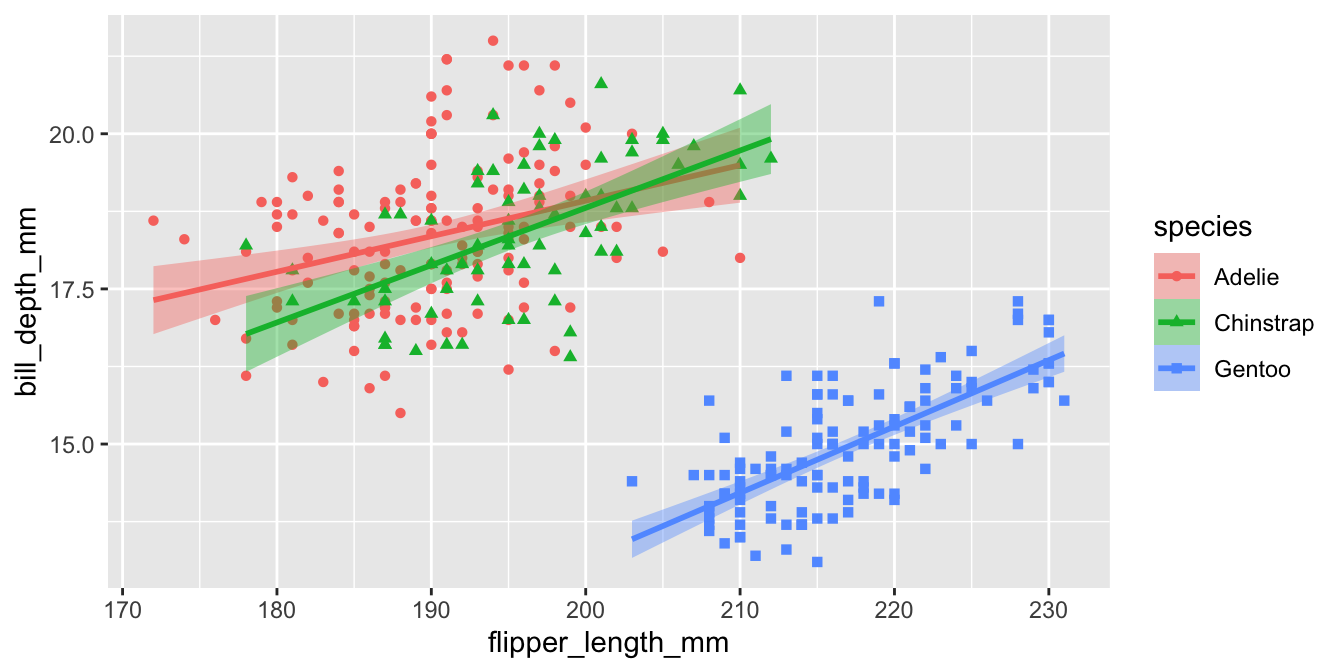
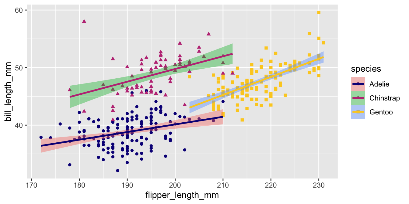
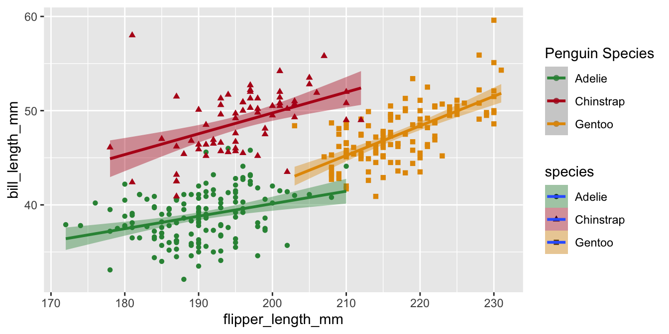
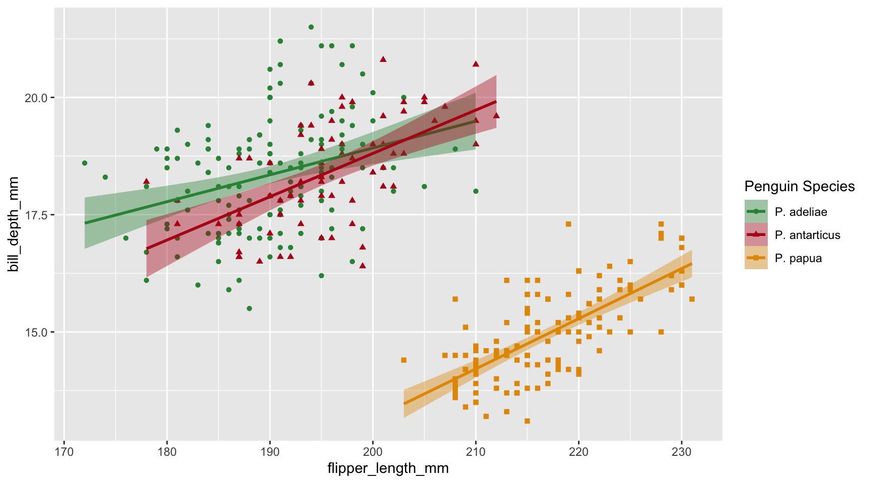
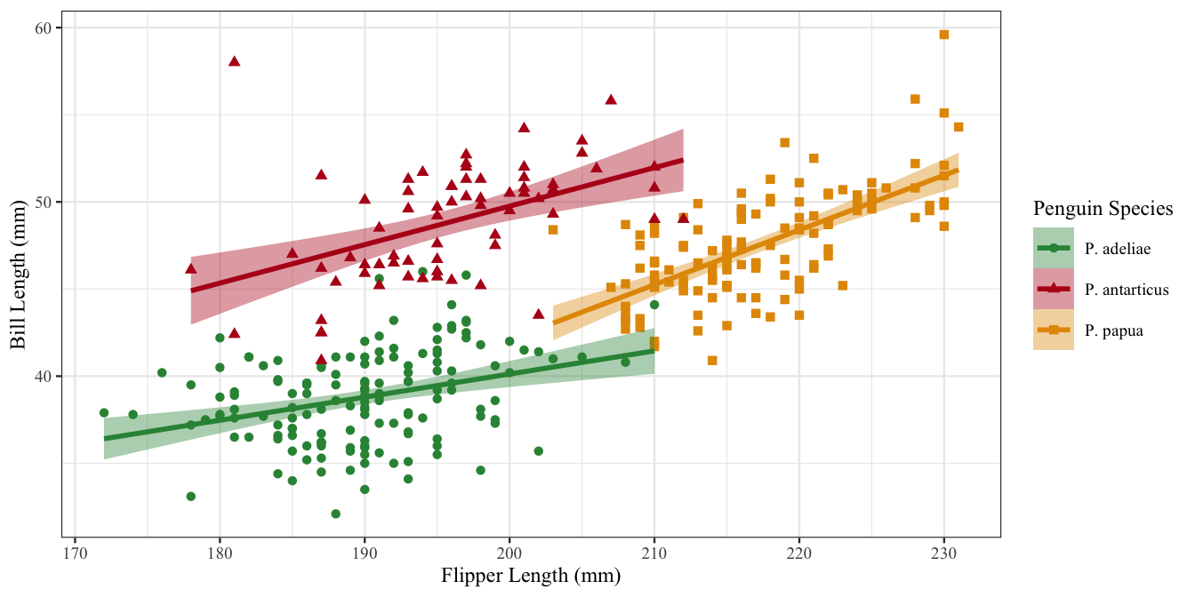
Example plot 2

p2 <-
  ggplot(penguins,
         aes(
           x = flipper_length_mm,
           y = bill_length_mm,
           color = species,
           fill = species,
           shape = species
         )) +
  geom_point() +
  geom_smooth(method = "lm")
p2

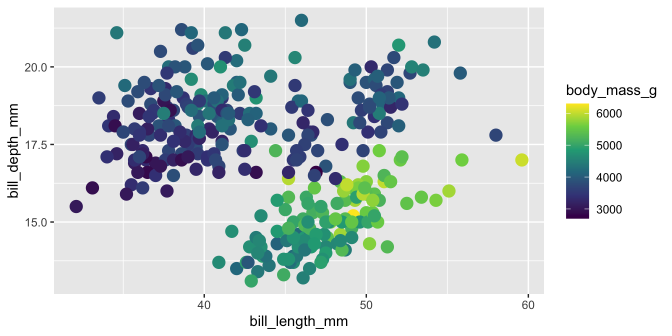
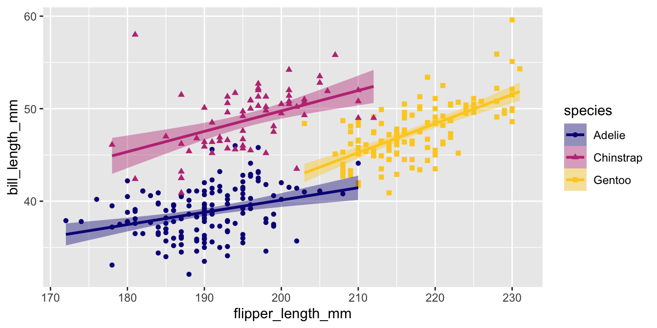
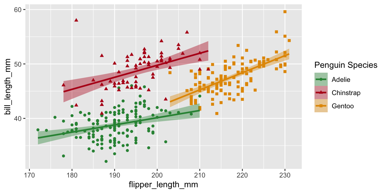
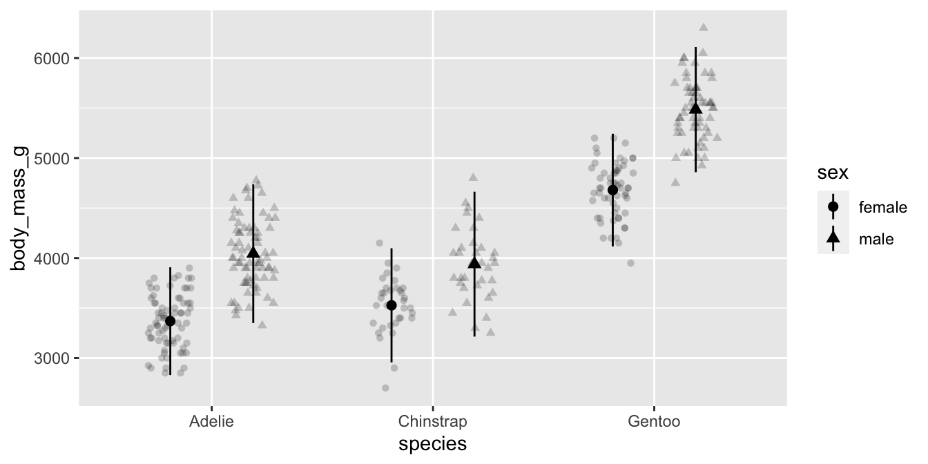
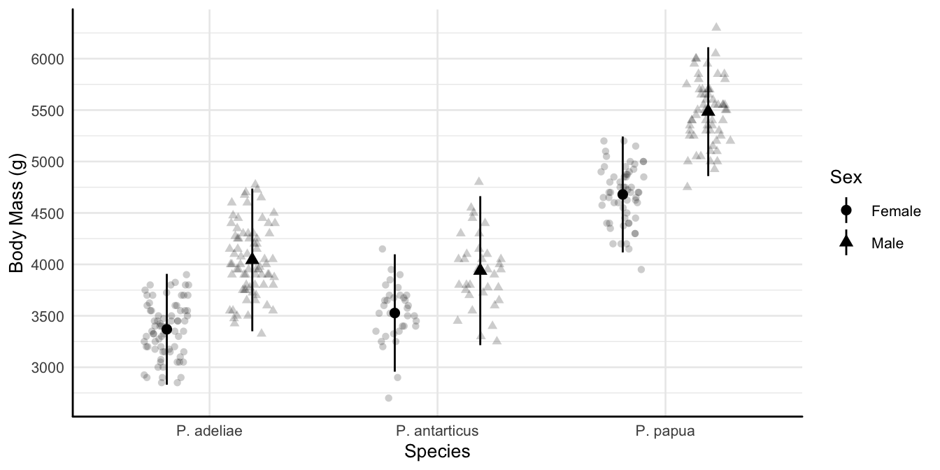
Example plot 3

p3 <-
  ggplot(penguins,
         aes(
           x = flipper_length_mm,
           y = bill_depth_mm,
           color = species,
           fill = species,
           shape = species
         )) +
  geom_point() +
  geom_smooth(method = "lm")
p3

Custom Colors

Color Palettes

Choose a color palette that is:

• Colorblind friendly
• Greyscale friendly
• Perceptually even
• High contrast (with background & within palette)

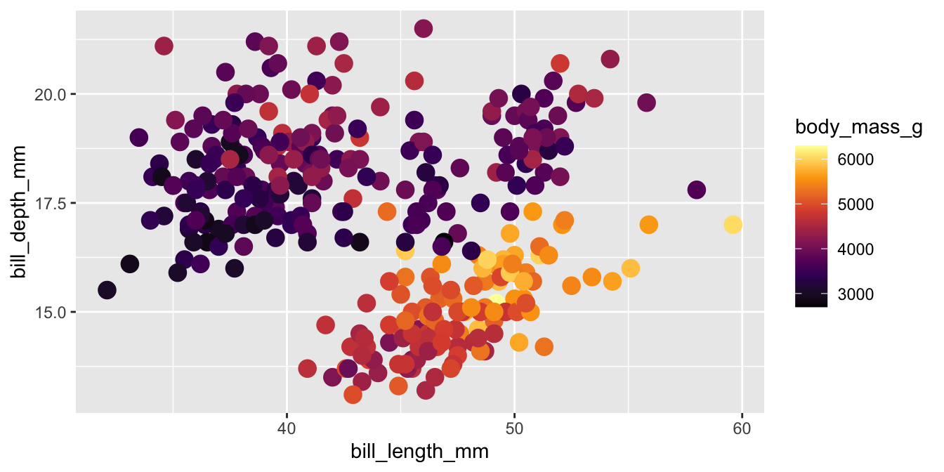
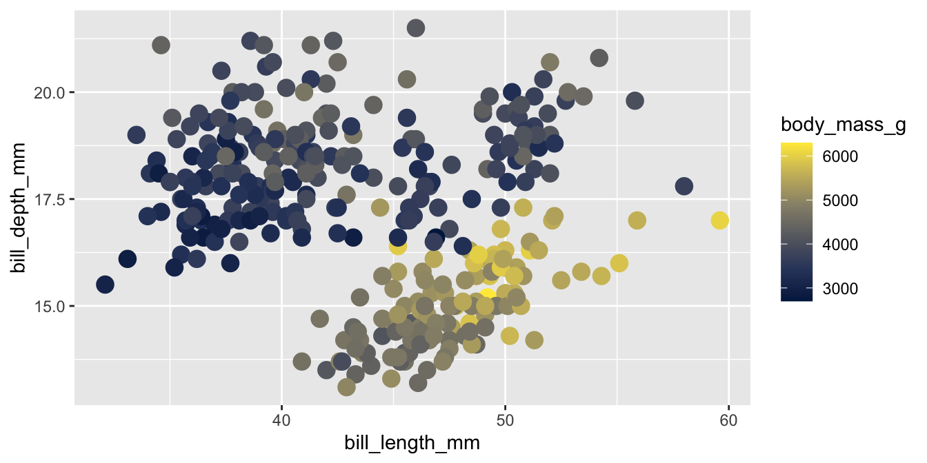
Viridis

The viridis color palettes meet most of these criteria and are built-in to ggplot2. They are available with scale_fill_viridis_*() and scale_color_viridis_*() functions.

v <- ggplot(penguins,
            aes(x = bill_length_mm, y = bill_depth_mm, color = body_mass_g)) +
  geom_point(size = 4)
v #default colors
v + scale_color_viridis_c() #viridis colors

Default color scale

Viridis color scale

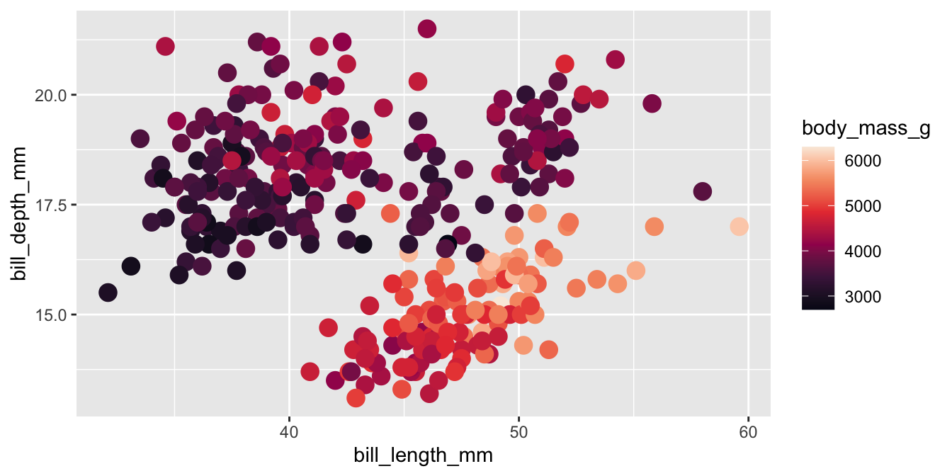
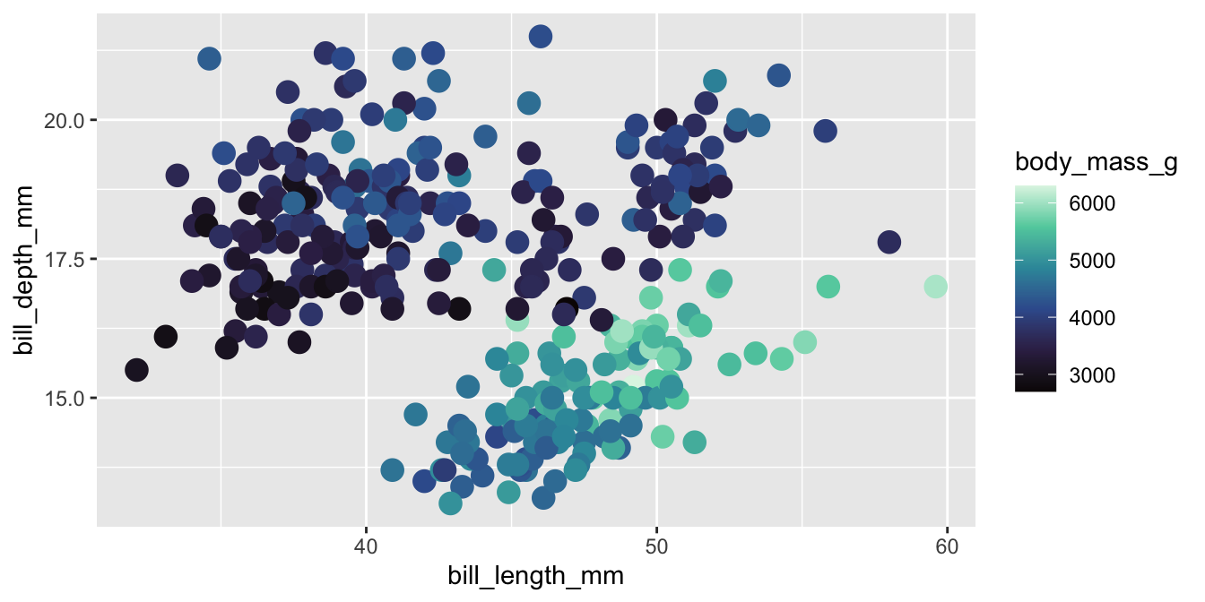
Viridis variants

Other viridis palettes are available by changing option in the scale function

Code

v + scale_color_viridis_c(option = "magma")
v + scale_color_viridis_c(option = "inferno")
v + scale_color_viridis_c(option = "plasma")
v + scale_color_viridis_c(option = "cividis")
v + scale_color_viridis_c(option = "rocket")
v + scale_color_viridis_c(option = "mako")

magma

inferno

plasma

cividis

rocket

mako

Viridis customization

The upper end of viridis palettes tends to be very bright yellow. You can limit the range of colors used with the begin and end arguments

v + scale_color_viridis_c()
v + scale_color_viridis_c(begin = 0.1, end = 0.9)

Viridis for discrete data

The viridis palette can be used for discrete / categorical data with scale_color_viridis_d().

p2 + scale_color_viridis_d(end = 0.9, option = "C")

Uh oh!

This only applied the new palette to the color aesthetic!

Applying palettes to multiple aesthetics

Usually color and fill are mapped to the same data. You can add both scale_color_*() and scale_fill_*() to a plot OR you can use the aesthetics argument.

p2 + 
  scale_color_viridis_d(aesthetics = c("color", "fill"), end = 0.9, option = "C")

Other color palettes

There are many places to get additional color palettes.

A few of my favorites:

• colorspace 📦
• cols4all 📦
• Comprehensive list of color palettes in r

Activity

Let’s find a palette we like using cols4all::4a_gui()

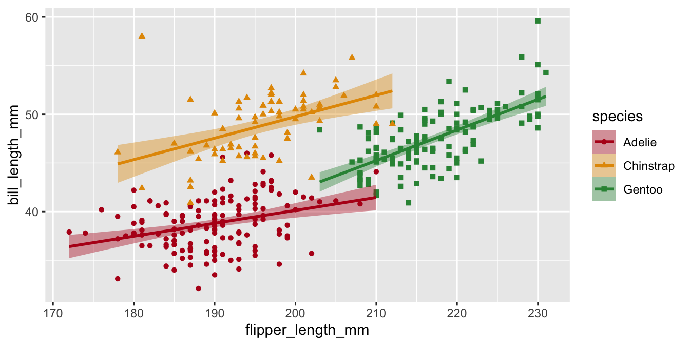
Manual color palettes

You can always use your own colors using scale_color_manual() if you know the hex codes.

my_cols <- c("#B60A1C","#E39802","#309143")

p2 + 
  scale_color_manual(values = my_cols, aesthetics = c("color", "fill"))

Manual color palettes

Use a named vector to specify which colors go with which factor level

my_cols <- 
  c("Chinstrap" = "#B60A1C", "Gentoo" = "#E39802", "Adelie" = "#309143")
p2 <- p2 + 
  scale_color_manual(values = my_cols, aesthetics = c("color", "fill"))
p3 <- p3 +
  scale_color_manual(values = my_cols, aesthetics = c("color", "fill"))

Legends

Legend titles

We can set the name for scales a few ways: with labs() or with the name= argument of the scale.

p2 + labs(color = "Penguin Species")

# Equivalent, but replaces existing color scale:
# p2 + scale_color_discrete(name = "Penguin Species") 

Legend titles

Legends for scales with the same name will be combined if possible

(p2 <- 
  p2 + labs(color = "Penguin Species",
            shape = "Penguin Species",
            fill = "Penguin Species"))

Legend titles

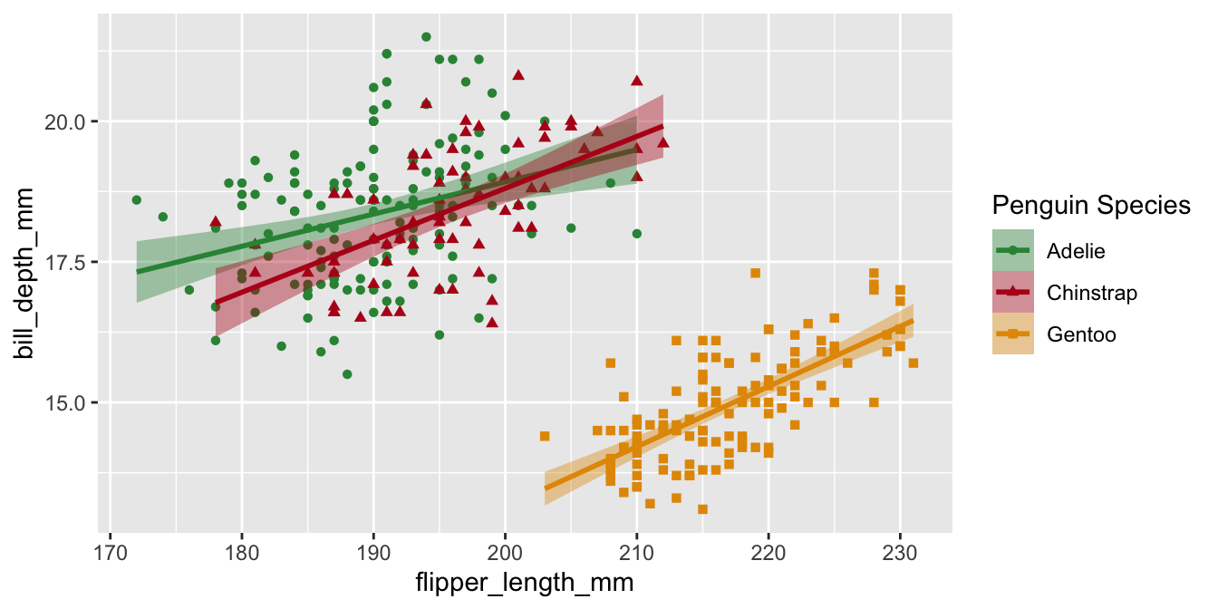
Let’s do the same for p3

(p3 <- 
  p3 + labs(color = "Penguin Species",
            shape = "Penguin Species",
            fill = "Penguin Species"))

Legend labels

What if we want to use the Latin name for the penguin species? We can use the labels argument and a named vector.

scinames <- c("Adelie" = "P. adeliae",
              "Chinstrap" = "P. antarticus",
              "Gentoo" = "P. papua")
p2 <- p2 +
  scale_color_manual(
    values = my_cols,
    labels = scinames,
    aesthetics = c("color", "fill")
  ) +
  scale_shape_discrete(labels = scinames)

p2

Legend labels

Legend labels

Let’s do the same for p3

p3 <- p3 +
  scale_color_manual(
    values = my_cols,
    labels = scinames,
    aesthetics = c("color", "fill")
  ) +
  scale_shape_discrete(labels = scinames)
p3

Tip

If there are many aesthetics that map to the same variable, it might be easier to change the factor levels in the data once instead of inside of every scale

Legend labels

Applying what we learned

Let’s apply what we learned to p1 to capitalize the words in the legend

• Which scale_ function?

• Which argument changes legend title?

• Which argument changes labels?

Applying what we learned

p1 <- p1 +
  scale_shape(
    name = "Sex",
    labels = c("male" = "Male", "female" = "Female")
  )
p1

Code auto-complete isn’t very helpful here because the only arguments to scale_shape() are … and solid. This is a good opportunity to talk about what … do and how to learn what arguments a function with … can take by looking at what function … are passed to in the help file.

Axes

Axes

Axes are also a type of scale. In p1 the x-axis corresponds to scale_x_discrete() and the y-axis corresponds to scale_y_continuous().

Custom labels

Use what we learned before to customize the categorical x-axis labels in p1!

(p1 <- p1 + scale_x_discrete(name = "Species", labels = scinames))

The nice thing about ggplot2 is that it is designed around a grammar—once you learn how to do something once, you can usually apply it easily to new situations.

Custom labels

If you only want to change the axis title, you can also do that in labs()

(p2 <- p2 + labs(x = "Flipper Length (mm)", y = "Bill Length (mm)"))
(p3 <- p3 + labs(x = "Flipper Length (mm)", y = "Bill Depth (mm)"))

Custom breaks

Change the (approximate) number of breaks with n.breaks=

(p1 <- p1 + scale_y_continuous(name = "Body Mass (g)", n.breaks = 12))

This uses “pretty” breaks at whole numbers, so you don’t get exactly n.breaks

Custom breaks

Specify breaks exactly with breaks=

p1 + scale_y_continuous(breaks = c(3333, 5000, 5555))

Themes

Complete themes

There are several complete themes built-in to ggplot2, and many more available from other packages such as ggthemes.

p2 + theme_bw()
p2 + theme_minimal()

theme_bw()

theme_minimal()

Fonts

You can customize font size and family with complete themes.

p2 + theme_bw(base_size = 9, base_family = "Times New Roman")

Custom themes

Customizing themes “manually” involves knowing the name of the theme element and it’s corresponding element_*() function.

p1 + theme(axis.title = element_text(face = "bold", colour = "red"))

Theme elements are hierarchical. E.g. title affects all title elements, axis.title affects all axis titles, axis.title.x only affects x-axis titles, and axis.title.x.bottom affects only the bottom x-axis title (in the case that there is a second x-axis on the top).

Custom themes

It’s best to find a built-in theme_*() function that gets you most of the way there and then customize with theme()

p1 + 
  theme_minimal(base_size = 10) + 
  theme(axis.line = element_line(linewidth = 0.5, lineend = "round"))

Custom themes

Activity

Name some things about the appearance of p1 that you want to change and we’ll figure it out together!

Tip

Check the examples in the help page for theme() https://ggplot2.tidyverse.org/reference/theme.html to figure out the names of theme elements

Re-using custom themes

You can save a custom theme as an R object and supply it to your plots.

my_theme <- 
  theme_minimal() + 
  theme(
    axis.line = element_line(linewidth = 0.5, lineend = "round"),
    axis.ticks = element_line(linewidth = 0.2),
    legend.background = element_rect(linewidth = 0.2)
  )

p2 + my_theme

Re-using custom themes

Or you can set your theme as the default at the top of your R script

theme_set(my_theme)
p3

Multi-panel figures

Combine plots

The patchwork package makes it easy to combine ggplot2 plots

library(patchwork)
p1 + p2

Control layout

• + wraps plots
• | combines plots horizontally
• / combines plots vertically
• () can be used to nest operations

p1 / (p2 | p3)

Multi-panel figures

• plot_layout(guides = "collect") combines duplicate legends
• plot_annotation(tag_levels = "a") adds labels to sub-plots

p_combined <-
  p1 /
  (p2 + p3 + plot_layout(guides = "collect")) + 
  plot_annotation(tag_levels = "a", tag_suffix = ")")
p_combined

Saving plots 💾

Saving plots

If you know the dimensions, it’s good to save plots early on and adjust theme to fit.

ggsave(
  filename = "penguins.png",
  plot = p_combined,
  width = 7, 
  height = 5, 
  units = "in", 
  dpi = "print",
  bg = "white"
)

The file type is figured out based on the extension in filename.

By default, the last plot is the one saved, but it’s good practice to specify plot anyways

Dimensions can be specified in pixels, inches, mm, etc.

dpi is resolution and only applies to raster images.

bg sets background color. If you don’t set this, the background of your plot is often transparent, which might not be the best for adding to presentations.

Notice how the legends and points look too large with these dimensions. It might be good to fix that.

Raster vs. Vector

• Raster images (e.g. .jpg, .png, .tiff) are made of pixels and the resolution can vary.
• Vector images (e.g. .svg, .eps) are not made of pixels and don’t have a resolution.
• Vector formats should be used whenever possible

Raster (72 dpi .png file)

Vector (.svg file)

Open images in a new tab and zoom in on browser to demo the difference.

Vector formats are not only resolution-less, they are more compatible with screen readers and therefore more accessible.

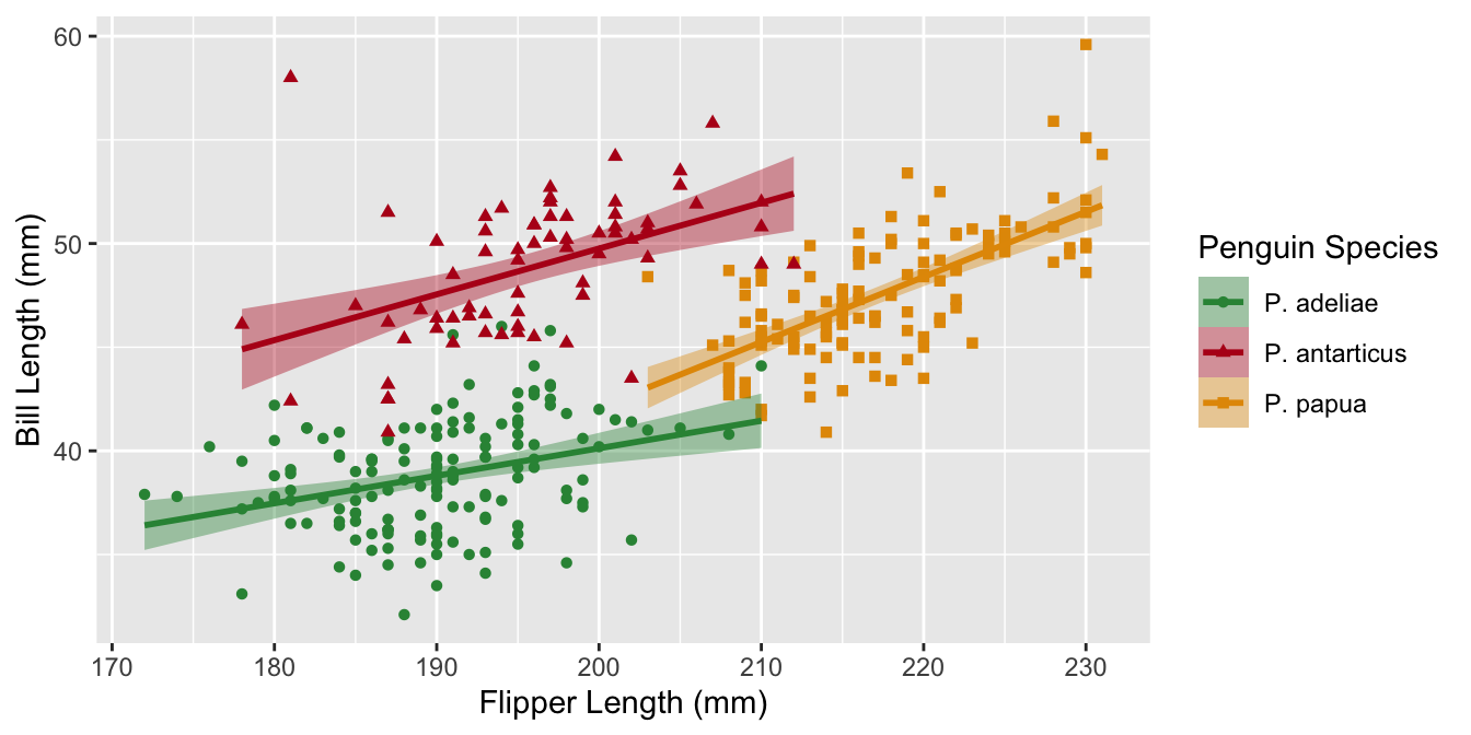
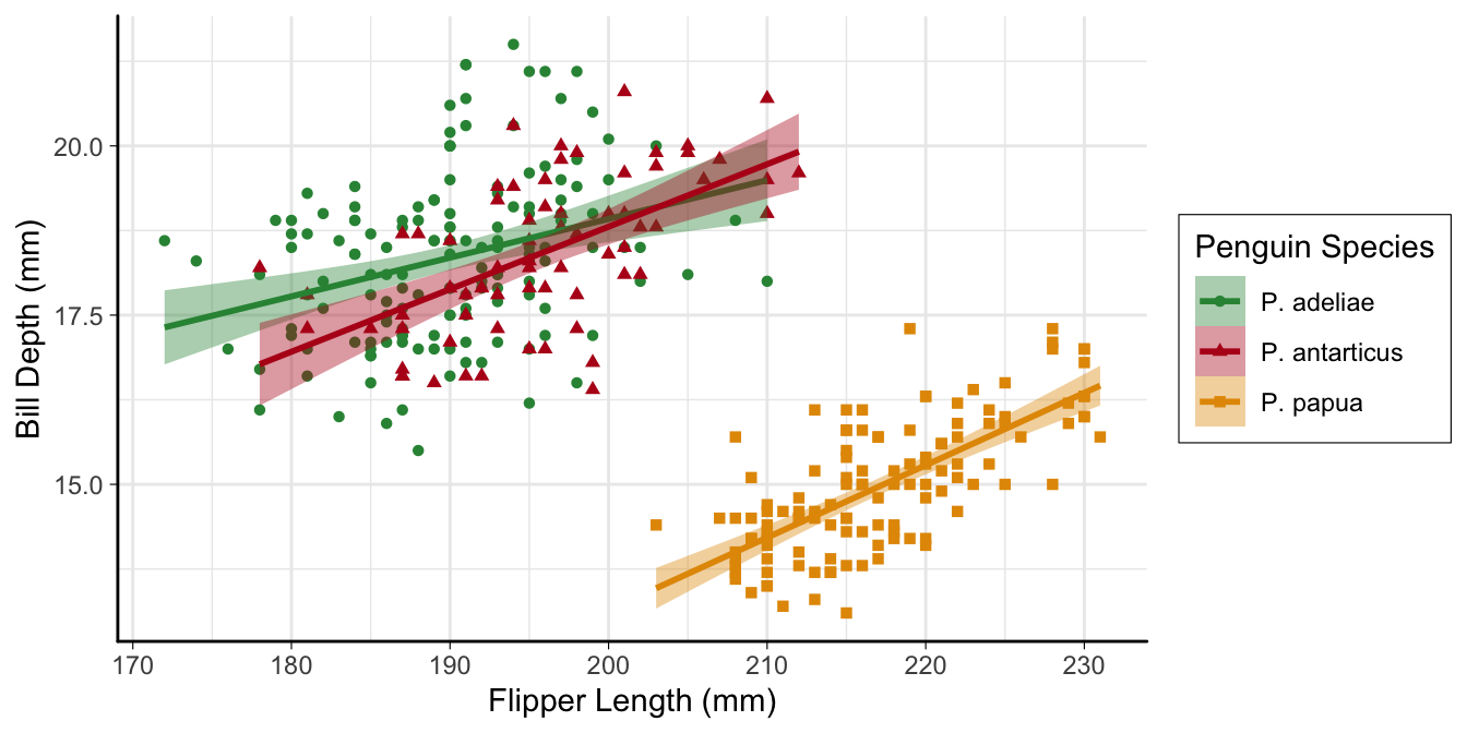
Finished product!

library(tidyverse) #includes ggplot2
library(palmerpenguins) #for data
library(patchwork) #multi-panel figures

# Custom theme
my_theme <- 
  theme_minimal(base_size = 10) + 
  theme(
    axis.line = element_line(linewidth = 0.5, lineend = "round"),
    axis.ticks = element_line(linewidth = 0.2),
    legend.background = element_rect(linewidth = 0.2)
  )
theme_set(my_theme)

# plot 1

## Custom function for stat_summary
mean_sd <- function(x) {
  data.frame(y = mean(x), ymin = mean(x) - sd(x), ymax = mean(x) + sd(x))
}

## For labeling with latin names
scinames <- c("Adelie" = "P. adeliae",
              "Chinstrap" = "P. antarticus",
              "Gentoo" = "P. papua")

p1 <-
  ggplot(penguins |> filter(!is.na(sex)),
         aes(x = species, y = body_mass_g, shape = sex)) +
  geom_point(alpha = 0.2,
             position = position_jitterdodge(dodge.width = 0.75)) +
  stat_summary(fun.data = mean_sd,
               position = position_dodge(width = 0.75)) +
  scale_x_discrete(labels = scinames) +
  scale_y_continuous(n.breaks = 12) +
  labs(x = "Species", y = "Body Mass (g)")

# Color palette for plot 2 and 3
my_cols <- 
  c("Chinstrap" = "#B60A1C", "Gentoo" = "#E39802", "Adelie" = "#309143")

p2 <-
  ggplot(penguins,
         aes(
           x = flipper_length_mm,
           y = bill_length_mm,
           color = species,
           fill = species,
           shape = species
         )) +
  geom_point() +
  geom_smooth(method = "lm") +
  scale_color_manual(
    values = my_cols,
    labels = scinames,
    aesthetics = c("color", "fill")
  ) +
  scale_shape_discrete(labels = scinames) +
  labs(
    color = "Penguin Species",
    shape = "Penguin Species",
    fill = "Penguin Species",
    x = "Flipper Length (mm)",
    y = "Bill Length (mm)"
  )

p3 <-
  ggplot(penguins,
         aes(
           x = flipper_length_mm,
           y = bill_depth_mm,
           color = species,
           fill = species,
           shape = species
         )) +
  geom_point() +
  geom_smooth(method = "lm") +
  scale_color_manual(
    values = my_cols,
    labels = scinames,
    aesthetics = c("color", "fill")
  ) +
  scale_shape_discrete(labels = scinames) +
  labs(
    color = "Penguin Species",
    shape = "Penguin Species",
    fill = "Penguin Species",
    x = "Flipper Length (mm)",
    y = "Bill Length (mm)"
  )

# combine into multi-panel figure
p_combined <-
  p1 /
  (p2 + p3 + plot_layout(guides = "collect")) + 
  plot_annotation(tag_levels = "a", tag_suffix = ")")

p_combined

Finished product!

Getting help

• The ggplot2 documentation itself, in particular the examples on the theme() page and the FAQ on customization.

• The R Graph Gallery has a wide variety of plots with R code walkthroughs.

• The ggplot2 book: https://ggplot2-book.org/

You can always come by our drop-in hours to ask questions as well!

Part 3 in two weeks!

“Exploring the wide world of ggplot2 extensions”

🗓️ June 26

⌚️ 11:00am–1:00pm

Registration